1.   Introduction

Generally, performance models for transportation infrastructure are divided into three categories, including empirical, mechanistic, and combined models (Hong and Prozzi, 2006; Luo, 2013; Wei et al., 2021). Rauhut et al. (1983) employed the mechanistic approach to develop a damage function for pavement rutting, fatigue cracking, and the loss of pavement serviceability index (PSI). However, a pure mechanistic approach is not suitable to directly establish a prediction model (Shahin, 2005). In the empirical approach, statistical techniques are used to estimate explanatory variables for facility deterioration, and this approach provides a method to relate the facility performance to its mechanical response. Therefore, numbers of mechanistic-empirical or empirical-mechanistic models have been proposed since then (Canestrari et al., 2022; Gong et al., 2023; Gu et al., 2017; Hasan et al., 2020; Ling et al., 2020; Luo et al., 2017; Prozzi, 2001; Timm et al., 2000; Yang et al., 2017; Zhao et al., 2017). Although the combined approach can take advantage of both mechanistic and empirical methods, it is not only complicated to calculate the result, but also difficult to update the model.

In many previous studies, performance models have been developed through the empirical approach in spite of its limitation associated with the scope and range of the available data. The polynomial constrained the least squares regression model, Markov or hidden Markov model (Cheng et al., 2019; Kobayashi et al., 2012), incremental model (Prozzi and Madanat, 2004), neural network model (Yang et al., 2006), survivor curve model (Wang et al., 2005), mixed effect model (Khraibani et al., 2012; Yu et al., 2007), time series or state-space specifications of multivariate time series model (Chu and Durango-Cohen, 2008; Durango-Cohen, 2007), and Bayesian model (Hong and Prozzi, 2006) are common practices of the empirical approach.

The lack of available data severely reduces the estimation precision, especially in the airfield pavement management. Therefore, it motivates the use of panel data for model. Panel data consist of two components: cross-section data and time series data. Cross-section data could describe the differences between the facilities comprising the panel (i.e., heterogeneity) and time series data, the evolution of individual facilities over time (i.e., serial dependence).

To address the heterogeneity, prediction models are often developed for "families". For instance, a pavement family is defined as a group of pavement monitoring sections with similar characteristics. Since sections in the same pavement family can still perform differently, several various approaches are proposed to estimate the individual section performance. The proportional augmentation method, which assumed that the deterioration rate of specific pavement is proportional to the one of family average, was proposed by Cook and Kazakov (1987). Shahin (2005) proposed a curve shifting method that draws the family prediction curve through the latest available condition. This method has been adopted in the PMS Micro PAVER. Then, linear mix effect models (LMEM) were introduced by Yu et al. (2007). The LMEM, the approach originally proposed by Henderson (1953), is also called the longitudinal model (Diggle, 1988). The distinguished feature of LMEM is the consideration of both family trend and individual condition history to predict future conditions. Usually, the mean response in LMEM is modeled as a combination of population characteristics shared by all individuals, and the subject-specific effects are unique to individuals. The former is regarded as a fixed effect, while the latter is considered a random effect. The mix effect models are denoted containing both fixed and random effects.

Most performance modeling approaches (Butler et al., 1985; Shahin, 2005) for panel data are static, which indicates that serial dependence cannot be captured, and performance models will not be updated with the new coming data. However, previous research has proven the significance of serial dependence. One solution to solve this problem is to use the structural time series (STS), auto regressive moving average approach (ARMA approach) or autoregressive moving average with eXogenous input (ARMAX) approach in the state-space form (Chu and Durango-Cohen, 2007; Civil Aviation Administration of China, 2009). The forecast process of models in state-space specifications are computed with a recursive algorithm called Kalman filter. Details on Kalman filter could be referenced to R. E. Kalman's article (Diggle, 1988). Ben-Akiva and Ramaswamy (1993) suggested that state-space models can rigorously address the problem of forecasting condition when multiple technologies are used to simultaneously collect various types of condition data. Another distinguished feature of the state-space approach is that the intervention analysis could be easily incorporated for performance jumps due to maintenance and rehabilitation (M & R) activities (Chu, 2013; Chu and Durango-Cohen, 2008). However, useful models should be able to quantify the effects of the most relevant variables on pavement deterioration (Prozzi and Madanat, 2004). STS, ARMA and ARMAX approach are not widely adopted due to its complexities in the incorporation of the exogenous explanatory variables, the external factors such as structural characteristics, environmental factors, and traffic (Chu, 2013; Chu and Durango-Cohen, 2008).

Methodological limitations mentioned in the previous paragraph motivated the development of state-space models to analyze time series with explanatory variables. Chu and Durango-Cohen adopted Ben-Akiva and Ramaswamy's framework and proposed a state-space approach including three specifications for multi-infrastructures' modeling problems, as shown in Eqs. (1) and (2) (Ben-Akiva and Ramaswamy, 1993; Chu and Durango-Cohen, 2008). Eq. (1) is the system equation which governs the infrastructures system deterioration and describes the effects of explanatory variables. The measurement equation is aimed to capture random errors during the inspection process. The three models, individual model, seemingly unrelated time series equation model, and single equation model, are considered in terms of the assumptions regarding the structure of underlying mechanisms generating the data sequence. These methods could well capture the heterogeneity and serial dependence. Moreover, this approach has successfully achieved the goal of dynamic performance prediction.

where X_{i, t} is the d-dimensional state vector representing the condition of facility i at the start of period t, Z_{i, t} is the k-dimensional observation vector representing the set of condition data/indicators collected for facility i in period t, A_{i, t} is the m-dimensional vector of exogenous explanatory variables, e.g., structural design, history of maintenance and rehabilitation activities, environmental factors, and traffic loading, g is the transition matrix, h is the explanatory variable, and the measurement matrix is the parameter that describes the effects of the above variables, Ω_t, Ξ_t are Nd- and Nk-dimensional Gaussian random vectors that capture disturbances/aleatory uncertainty in the deterioration and inspection processes, respectively.

China's inspection system for airport pavement damage was not officially established until 2009. Previously, only a few Chinese airports have conducted inspections for their pavements, and all airports in China have not experienced more than five thorough pavement inspection works so far. The inspection data are regarded as panel data which contain a large number of data on individual facilities, but few observation data over time. The characteristics of these data set indicate that the performance modeling method proposed by Durango-Cohen is not suitable. To address this problem, PDMs including the LMEM are introduced. In this study, static and dynamic PDMs in state-space forms are proposed to formulate dynamic performance for transportation facilities and are estimated using the panel data. Two regression methods, the ordinary least square (OLS) and the generalized method of moments (GMM), are employed for estimation and comparison.

2.   Methodology

2.1   Static panel models and analysis

2.1.1   Static entity fixed effects models (S-EFEM)

Fixed effects model includes an entity fixed effects model (EFEM), a time fixed effects model, and a time and entity fixed effects model. Due to the short period of longitudinal data, only EFEM is selected for the estimation in this study. In terms of the entity fixed effects model, the intercept of the model is different for individuals, but the intercept does not change significantly for different cross-sections. The S-EFEM's specification can be represented as shown in Eqs. (3) and (4).

In Eq. (3), c and α_i is the intercept owned by all individuals and section i, respectively. Pavement sections are assumed not to interact with each other, but with the deterioration induced by one exogenous variable, therefore block diagonal matrix of g and h. Also, the structures of Eq. (4) have two implications. If Var(Ω_t) is block diagonal, only cross-sectional heteroscedasticity is considered in the specification. This denotes that the heterogeneity is captured by the disturbance term of individual. If Var(Ω_t) is not block diagonal, cross-sectional correlation would also be considered. However, the consideration of cross-sectional correlation is only practical with a small number of sections. To reduce the number of estimating parameters, cross-sectional correlation of measurement equation would not be considered in all the proposed models as shown in Eq. (4).

2.1.2   Static entity random effects model (S-EREM)

Similarly, the random effects model also includes an entity fixed effects model, a time random effects model and a time and entity random effects model. Also, only entity random effects models are selected for the estimation. The S-EREM's specification can be represented as an instance of general state-space model as shown below in Eqs. (5)-(7)

Compared to S-EFEM, the distinguished feature of S-EREM is that symbols α_i and Ω_{i, t} listed in Eq. (7) are random variables assumed to be independent and identically distributed (IID), but not limited to their distributions. Moreover, α_i has no relevance to X_{i, t} and Var(Ω_t) is not block diagonal.

2.2   Dynamic panel models in state-space specifications

In this section, three classes of dynamic panel data models are presented, including dynamic entity fixed effects model (D-EFEM), D-EREM, and dynamic linear mixed effects model (D-LMEM). The distinguished feature of dynamic panel models is a lag observation vector in the expression which makes the models capable of using state-space specifications.

2.2.1   Dynamic entity fixed effects model (D-EFEM)

Like the static panel data models, entity fixed effects models are also selected for the estimation. The specification of D-EFEM can be represented as an instance of general state-space model as shown below in Eqs. (8)-(11).

The variables here are identical to those in Eqs. (3) and (4).

2.2.2   Dynamic entity random effects model (D-EREM)

Also, only entity random effects models are selected for the estimation. The specification of D-EREM can be represented as an instance of general state-space model as shown below in Eqs. (12)-(16).

The variables here are identical to those in Eqs. (5) and (6).

2.2.3   Dynamic linear mixed effects model (D-LMEM)

If any individual and cross-section do not exhibit significant differences, the LMEMs are applicable and can be regarded as a good model. Two types of LMEMs are presented: D-LMEM1 with the intercept and D-LMEM2 without the intercept. D-LMEM1 is presented in Eqs. (17)-(20). It could be seen that parameters are area independent in this formulation. The individual heterogeneity among the areas is expressed by the individual error term Ω_{i, t}.

All the variables seem physically meaningful except the intercept c when taking a view at the formulation. For instance, if A_{i, t} represents the traffic loading and then h could be explained as the influence of traffic on performance deterioration. Therefore, the measurement equation of D-LMEM2 is formulated without the intercept as shown in Eq. (21). The rest equations are identical to those of D-LMEM1.

3.   Results and discussion

3.1   Empirical study

3.1.1   Data set

Pavement performance deterioration is estimated using a panel of 7 sections from the runway in Shanghai Hongqiao International Airport. This airport is located in east China and has two runways now. The first runway, the studied runway, has been refurbished by asphalt mixture overlays for several times. The airport agency has monitored and measured the PCI conditions for the first runway by means of visual inspection conducted by trained staff since 1998 and obtained 9 groups of data. In this study, the inspection data between 1999 and 2005 are used for the models' estimation, and the data between 2008 and 2010 are used for the models' comparison.

3.1.2   Explanatory variables

The models presented in the previous section require variables of distress measurements and explanatory variables. X_{i, t} is the state variable representing the pavement condition index (PCI) value of section i at time t. The survey assessment was performed following the guidelines provided in the Pavement Condition Rating Manual (Civil Aviation Administration of China, 2009). Tr_{t, i} is the annual weighted traffic loading burdened by section i at time t measured in 10³ equivalent traffic for the design aircraft, B747-400. This variable is used for dynamic panel models while STr_{t, i} for static panel models. The convention equation for aircraft k is shown in Eq. (22). Then the sum of all aircrafts' equivalent traffic would be the final annual weighted traffic.

where N_s is the equivalent traffic of the aircraft k for the design aircraft s, δ is the convention parameter of the main gear, N_k is the annual traffic for the aircraft k requiring convention, P_k is the main gear's load of the aircraft k requiring convention, P_s is the main gear's load of the design aircraft s, SumTr_{t, i} is the sum of weighted traffic loading burdened by section i in t years measured in 10³ equivalent traffic for the design aircraft, B747-400. Annual weighted traffic loading burdened by section i at time t are referenced to the computation of Tr_{t, i}, Th_{t, i} is the structural number of the section i at time t. A pavement's structural number serves as an input for its structural design. For the composite pavement, the equivalent thickness of each pavement layer could be calculated by Eq. (23) (Civil Aviation Administration of China, 2009).

where h_e is the effective thickness of composite pavement, C_F and C_R are the reduction factors of asphalt (Portland cement concrete, PCC) pavement, h_F and h_R are the thicknesses of asphalt (PCC) pavement (F means flexible pavement and R means rigid pavement), F is the factor related to the pavement distress condition. It is widely believed that the pavement of more serious damage would suffer more damage for the same traffic loads. Here, it is defined as a function of PCI as shown in Eq. (24) with reference to the evaluation of PCI (Civil Aviation Administration of China, 2009). As it can be seen from Eq. (24), equivalent pavement thickness is varying with the deterioration condition, which is of significant difference compared with the previous research. Table 1 shows the pavement structure and calculation procedure of the effective thickness of each layer at the runway's refurbished year marked in brackets.

Table  1.  Effective thickness of each layer at the refurbished year.

Section	Layer	Thickness (cm)	Reduction factor	Effective thickness (cm)	Cumulative effective thickness (cm)
R2, R3, R7, R8	Asphalt overlay (05)	7.0	1.00	7.0×0.4=2.8	40.9 = 38.1 + 2.8
	Asphalt overlay (98)	7.5	0.80	6.0×0.4=2.4	38.1 = 35.7 + 2.4
	Asphalt overlay (91)	14.0	0.75	10.5×0.4=4.2	35.7 = 31.5 + 4.2
	PCC concrete	45.0	0.70	31.5	31.5
R4, R5, R6	Asphalt overlay (05)	7.0	1.00	7.0×0.4=2.8	38.1 = 35.3 + 2.8
	Asphalt overlay (98)	7.5	0.80	6.0×0.4=2.4	35.3 = 32.9 + 2.4
	Asphalt overlay (91)	14.0	0.75	10.5×0.4=4.2	32.9 = 28.7 + 4.2
	PCC concrete	41.0	0.70	28.7	28.7

下载: 导出CSV 

| 显示表格

where OV_{t, i} is the variable to incorporate the overlay effects into the formulation. It is assumed that if the overlay is adopted, the PCI will arrive at 100, the full score.

3.1.3   Models' estimation results

Five classes of models and their six instances mentioned above are considered for estimation. S-EFEM, S-EREM, D-EFEM, D-EREM, D-LMEM1 and D-LMEM2 are modeled with the above-mentioned variables. The S-EREMs and S-EFEMs are estimated using OLS. Then the Hausman Test is conducted to choose a better one from the two static alternatives.

For the dynamic counterpart, OLS can also be used for the parameter estimation. However, the existence of the lagged dependent variables between the regressors can cause the endogeneity problem. This endogeneity problem associated with dynamic models is tackled using the generalized method of moments (GMM) procedure which is proposed by Arellano and Bond (1991), and GMM is proved more efficient than the instrumental variable (Ⅳ) estimation procedure suggested by Anderson and Hsiao (1982). Arellano and Bond (1991) demonstrated additional instruments can be obtained in a dynamic panel data model if one utilizes the orthogonality conditions that exist between lagged values of the dependent variable and the disturbances. Using these moment conditions, Arellano and Bond (1991) proposed a two-step difference GMM (DGMM) estimator. And then the system-GMM (SGMM) estimator is developed by Blundell and Bond (1998). Following good practice guidelines suggested by several authors, notably, it is better to avoid DGMM estimation for an unbalanced panel. DGMM estimation approach has a weakness of magnifying gaps (Roodman, 2009). The panel used in the section of Empirical Study is close to be balanced, but again it is wise to avoid DGMM estimation. In some cases, so called "orthogonal deviations" can be used to "fill" missing gaps by subtracting "the average of all future available observations of a variable" (Roodman, 2009). The estimate of the model specification including orthogonal deviations does not provide better statistical diagnostics in comparison to SGMM. Therefore, SGMM is preferred for comparison with OLS.

The summary of the estimation results is shown in Table 2, and the final PCI specifications are presented in Eqs. (26)-(32). OLS and SGMM are estimated using statistical software R and Stata, respectively. It should be noted that since P = 0.0319 and the confidence level of the Hausman test is 0.05, it obviously rejects the hypothesis of random effect components, so the results of the random effect model are ignored, as shown in Table 2.

Table  2.  Estimation results.

Model	Variable	Xt, i	Trt, i (STrt, i)	Tht, i	MSt, i	CPt, i	MRt, i	PTi	C
S-EFEM (OLS)	Coefficient	−6.568	2.917	8.740	11.451	22.301	27.178	0.435	−6.568
	SE	4.905	0.584	3.537	3.121	3.718	6.869	0.136	4.905
	t-statistic	−1.34	4.99	2.47	3.67	6.00	0.62	2.31	−1.34
	P	0.213	0.001	0.035	0.005	0	0.550	0.362	0.213
	R/AIC/SSE	0.850/4.125/39.042
D-EFEM (OLS)	Coefficient	0.133	−10.211	2.508	1.954	1.314	1.417	0.334	35.869
	SE	1.99	7.06	6.03	1.36	0.55	0.41	0.215	9.17
	t-statistic	0.0671	−0.6358	0.4160	1.4422	2.3972	3.4782	3.6200	0.5590
	P	0.9482	0.5426	0.6884	0.1872	0.0434	0.0083	0.4530	0.5915
	LL/AIC/SSE	−32.862/4.368/28.117
D-EREM (OLS)	Coefficient	0.836	−5.322	0.405	6.108	9.323	19.746	0.385	22.182
	SE	0.245	4.300	0.421	3.403	2.803	3.240	0.337	8.057
	t-statistic	3.4130	−0.5723	0.9614	1.7947	3.3266	6.0945	2.8600	0.4029
	P	0.0042	0.5762	0.3527	0.0943	0.0050	0	0.1950	0.6931
	LL/AIC/SSE	−/−/36.103
D-LMEM1 (OLS)	Coefficient	0.843	−5.201	0.394	6.019	9.313	19.816	0.415	21.326
	SE	0.210	6.250	0.330	3.000	2.480	2.850	0.219	7.800
	t-statistic	4.0637	−0.6305	1.2082	2.0032	3.7515	6.9490	3.9200	0.4372
	P	0.0012	0.4385	0.2470	0.0649	0.0021	0	0.1200	0.5686
	LL/AIC/SSE	−36.309/4.125/39.042
D-LMEM2 (OLS)	Coefficient	0.903	−1.726	0.384	4.906	8.599	19.583	0.411	–
	SE	0.152	2.147	0.317	1.554	1.818	2.725	0.226	–
	t-statistic	5.9589	−0.8039	1.2115	3.1580	4.7283	7.1872	3.7900	–
	P	0	0.4340	0.2444	0.0065	0.0003	0	0.0120	–
	LL/AIC/SSE	−36.451/4.043/39.575
D-LMEM1 (SGMM)	Coefficient	0.718	−7.836	0.489	6.959	9.454	19.125	0.436	41.642
	SE	0.798	4.112	0.732	2.445	1.623	2.621	0.147	8.057
	t-statistic	0.900	−0.430	0.670	1.080	3.750	3.660	3.550	11.591
	P	0.403	0.680	0.529	0.322	0.010	0.011	0.041	0.761
	ST/HT	0.250(0.614)/0(1.00)
D-LMEM2 (SGMM)	Coefficient	0.969	−2.201	0.277	4.920	9.022	20.320	0.328
	SE	0.128	2.712	0.191	1.166	2.448	4.370	0.051
	t-statistic	7.55	−0.81	1.45	4.22	3.68	4.65	4.21
	P	0	0.444	0.190	0.004	0.008	0.002	0.003
	ST/HT	0.40(0.8)/1.40(0.497)
Note: SE is standard error, R2 is adjusted R2, AIC is akaike information criterion, SS is one-step prediction sum of square errors, LL is log likelihood, ST is Sargan test, HT is Hansen test, MSt, i is the indicator variable where, MSt, i  = {1, when micro surfacing is applied on section i between t and t+1; 0, otherwise}, CPt, i is the indicator variable where, CPt, i  = {1, when crack pouring is applied on section i between t and t+1; 0, otherwise}, MRt, i is the indicator variable where MRt, i  = {1, when major repair is applied on section i between t and t+1; 0, otherwise}, PTi is the indicator variable of different pavement type where PTi = {1, cement pavement; 0, asphalt pavement}.

下载: 导出CSV 

| 显示表格

S-EFEM(OLS)

D-EFEM(OLS)

where α₁=−1.23, α₂=−3.48, α₃=3.66, α₄=3.15, α₅=2.12, α₆=−1.42, α₇=−2.80, Z_{t, i}=X_{t, i}+Ξ_t, Ξ_t~N(₀, 7.38²).

D-EREM(OLS)

where α₁=0.25, α₂=−0.23, α₃=0.19, α₄=0.06, α₅=−0.26, α₆=0.16, α₇=−0.17, Zt, i=Xt, i+Ξt, Ξt~N(₀, 1.27²).

D-LMEM1(OLS)

where Z_{t, i}=X_{t, i}+Ξ_t, Ξ_t~N(0, 1.36²).

D-LMEM2(OLS)

where Z_{t, i}=X_{t, i}+Ξ_t, Ξ_t~N(0, 1.37²).

D-LMEM1(SGMM)

where Z_{t, i}=X_{t, i}+Ξ_t, Ξ_t~N(0, 1.37²).

D-LMEM2(SGMM)

whereZ_{t, i}=X_{t, i}+Ξ_t, Ξ_t~N(0, 1.26²).

Except for D-EFEM, the results in Table 2 do not show a significant difference between the models, but in fact, the maintenance effect of the three methods, micro surfacing, pavement sealing, and major repair, should be significantly different based on engineering experience. However, the estimation results of D-EFEM could not reflect this point while the others could. It could be seen that the D-EFEM obtains a lower SSE, but with consideration of AIC and LL, D-LMEM1 and D-LMEM2 using OLS are of better estimation. Generally, F-test could be used to judge whether to reject the hypothesis of non-significance of the fixed effects. In this case, F-test with the confidence level of 0.95 also clearly rejects the hypothesis of fixed effect components (F=0.081 < F_0.95(7, 14)=2.76).

To see if over identifying assumptions hold in instrumental variable estimation, the Sargan test is conducted when using SGMM for variables' estimation. The Sargan test results of both D-LMEM1 and D-LMEM2 are not stable. Moreover, the intercept's estimation of D-LMEM1 is not significant. Considering the limited available data, the two models may still be suitable for performance forecast. For instance, in the D-LMEM2, the parameters' estimates of X_{t, i}, MS_{t, i}, CP_{t, i} and MR_{t, i} are of high significance (P values are less than 0.05). The estimation results highlight the benefits of intervention analysis to represent the effects of maintenance activities. It is worth noting that only a particular (non-random) subset of samples is used to estimate effectiveness of each activity, which can result in selectivity bias. Maintenance effects would be more convenient for estimation with a relatively large panel of data. Luckily, the maintenance activities in sample airport are adopted at a small range of PCI (74–90), which could reduce the selection bias. This may also be the main reason why variables have a high significance on the estimation of maintenance effects.

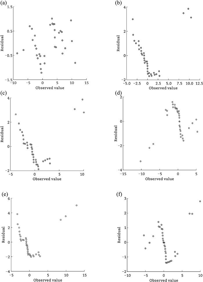
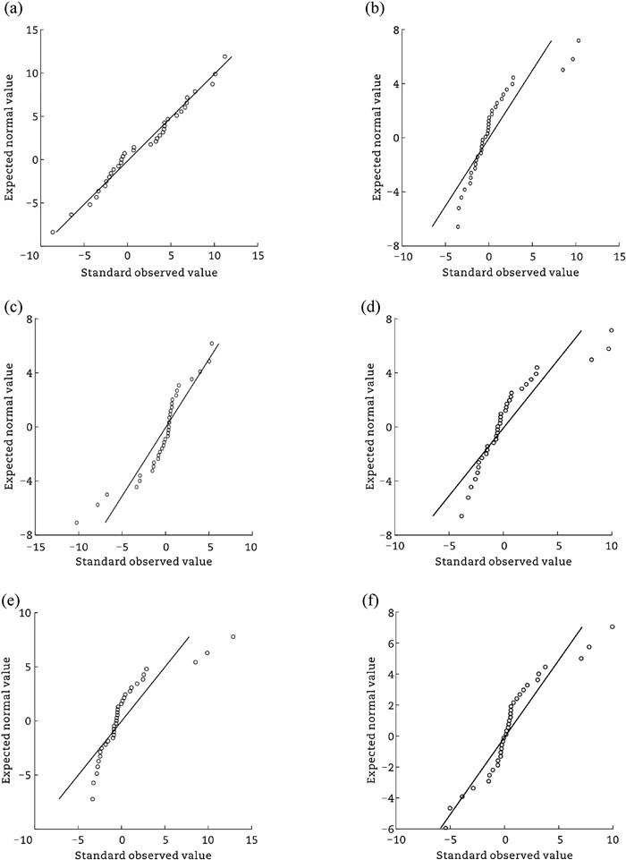
Therefore, the computed instances except D-EFEM are selected for the further analysis. The normality of the measurement errors was checked using the normal quantile-quantile (QQ) plot of the residuals in Fig. 1. Fig. 1 indicates that there is no significant deviation from the normality assumption, and Fig. 2 shows the distribution of the residual error.

Figure  1.  Normal QQ plot of models' residuals. (a) S-EFEM. (b) D-EREM. (c) D-LMEM1(OLS). (d) D-LMEM2(OLS). (e) D-LMEM-1(SGMM). (f) D-LMEM2(SGMM).

下载: 全尺寸图片 幻灯片

Figure  2.  Distribution of models' residuals. (a) S-EFEM. (b) D-EREM. (c) D-LMEM1(OLS). (d) D-LMEM2(OLS). (e) D-LMEM-1(SGMM). (f) D-LMEM2(SGMM).

下载: 全尺寸图片 幻灯片

3.1.4   Model comparison

Fig. 3(a) shows the section-average RMSE (root mean square error) of three years. The static model S-EFEM obtains lower accuracy than the other dynamic models, and the estimation results of D-LMEM2 using either OLS or SGMM are more accurate in prediction. Fig. 3(b) shows the section-average RMSE per year. It is obvious that almost every section-average RMSE of state-space models is less than that of S-EFEM. It should be noted that these dynamic models can achieve a relatively low RMSE (≤2) in the third year after resurfacing, and these dynamic models successfully meet the accuracy requirements in engineering practice.

Figure  3.  Comparison of models' estimation results. (a) Comparison of models' section-average RMSEs. (b) Comparison of models' section-average RMSES per year.

下载: 全尺寸图片 幻灯片

As mentioned earlier, both OLS and SGMM are used for the parameter estimation of D-LMEM1 and D-LMEM2. Although SGMM can provide an unbiased estimation result, its estimation results in this case seem not to be more accurate than OLS when used for performance prediction as shown in both Fig. 3(a) and (b). It can be concluded that in this case, the intercept c should be eliminated when formulating LMEM because the prediction accuracy of D-LMEM1(OLS) and D-LMEM1(SGMM) is better than D-LMEM2(OLS) and D-LMEM2(SGMM), respectively.

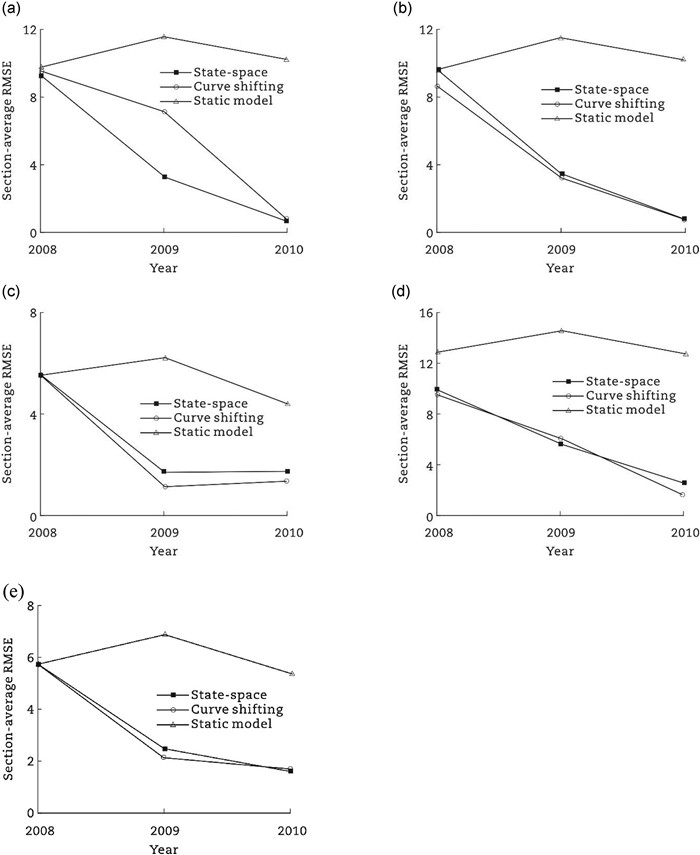
As discussed earlier, one of the distinguished features of dynamic models is that the models could be updated with the new coming data. In fact, in addition to the state-space models, some other methods can also be used to update dynamic models, including the curve shifting method. Here, the prediction results of the state-space method, curve shifting method, and static counterparts (new data are not used for update) are compared as shown in Fig. 4. Fig. 4 shows that each section-average RMSE of either state-space model or curve shifting model is less than those of its static counterpart. The section-average RMSE of the static model and the dynamic models decreases as the prediction continues over time, indicating the priority of dynamic performance modeling. It can be concluded that, to ensure the prediction accuracy, periodic inspections are required for the infrastructure management to update performance predictions.

Figure  4.  Three methods' comparison on section-average of RMSE per year. (a) D-EREM. (b) D-LMEM1(OLS). (c) D-LMEM2(OLS). (d) D-LMEM1(SGMM). (e) D-LMEM2(SGMM).

下载: 全尺寸图片 幻灯片

Moreover, no significant difference in prediction accuracy is found between state-space model and curve shifting model as shown in Fig. 4. Ordinarily, under the assumption of normal distribution disturbances and state vectors, the state space models are related to providing optimal estimate of the system through recursive maximum likelihood estimation. Therefore, to obtain accurate estimates, more inspection data may be needed, rather than just three groups.

3.2   Discussion on nonlinear models

Unfortunately, none of the proposed models could capture the combined effects between variables. For example, it is known that thicker pavements would suffer less damage under the same traffic loads. However, the LMEM could not express this phenomenon. Nonlinear mix effect model (NLMEM) is natural extension for LMEM and can process repeated measurement data through nonlinear formulas. Therefore, NLMEM was employed to solve the problem. Khraibani et al. (2012) adopted the NLMEM for the pavement performance modeling. However, the NLMEM model is static. Here, the state-space form of NLMEM without the intercept would be presented as shown in Eq. (33) for the dynamic modeling.

It can be seen from Eq. (33) that the parameter of A_{i, t} are set as functions of constant variables. During the modeling process, the specifications could be formulated in any forms without violating the structure of the state-space model or the estimating procedure. The rest equations are identical to those of D-LMEM1. It is worth noting that NLMEM could handle the nonlinear relationship lying between variables, but due to its complex form, NLMEM estimates require more data than LMEM. In many cases with few data available, LMEM could be a better option which leads to reliable estimation of variables.

In this case, with reference to Chu and Durango-Cohen (2008), the formulation of NLMEM can be formulated as shown in Eqs. (34), (35). The effects of Th_{t, i} is included in the NLMEM specification through a nonlinear transformation.

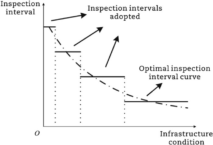
The estimation was also performed with the statistical software R and its library (NLME). However, due to the lack of available data, NLMEM could not be estimated. The foregoing discussion has proven that the availability of data is the main challenge of applying the proposed approach. The latest developments in remote sensing and communication technology can assist in regular inspections of transportation infrastructure. Since the previous research has shown the optimal inspection interval varies with infrastructure conditions, it is recommended to classify the inspection interval into several constants for various infrastructure conditions through this case, as shown in Fig. 5. This is due to that parameter estimation of dynamic PDMs requires continuous time series data within a certain inspection interval. In addition, this strategy facilitates the management of infrastructure agencies. Obviously, the difference in the inspection interval makes it impossible to use life cycle data for performance modeling unless the intervals are set by an integer multiple relationship. Therefore, it is recommended to check the integer multiple relationship between intervals.

Figure  5.  Inspection strategies suggested.

下载: 全尺寸图片 幻灯片

4.   Conclusions

In this study, the state-space specification of dynamic PDMs are proposed to formulate the dynamic performance model for transportation facilities and panel data sets are used for estimation. This framework provides a flexible and rigorous approach to capture the heterogeneity and update forecast through inspection simultaneously. PDMs are applied to tackle the cross-section heterogeneity of longitudinal data, and PDMs in state-space forms are used to achieve the goal of updating performance forecast with the new coming data. The results highlight the benefits of pooling data across facilities but due to the lack of data, some parameter estimates are not significant. There is no significant deviation between residuals and the normality assumption. The following conclusions can be drawn.

(1) By comparing the estimated models, the results prove that the state-space models could obtain more accurate predictions through inspection over time.

(2) Compared with the curve shifting method and the static model, there is no significant difference in prediction accuracy between the state-space model and the curve shifting model within a short period. It is strongly recommended that the inspection should be conducted to update the forecast of state-space formulations to guarantee the prediction accuracy.

(3) In practical engineering, the prediction accuracy of SGMM is not much different from that of OLS due to the lack of data.

(4) Although it is in possible to obtain parameter estimates in this empirical study, it is still suggested to use NLMEM for the performance prediction to handle the potential nonlinear relationships with a suitable data set.

(5) Compared to the fixed inspection strategy, the dynamic inspection strategy could not only save costs, but also make inspection results more accurate. Inspection intervals are suggested to be specified as several constants with an integer multiple relationship.